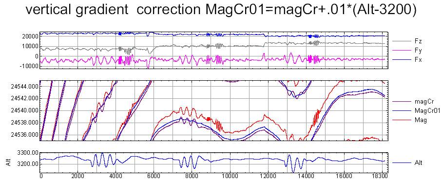
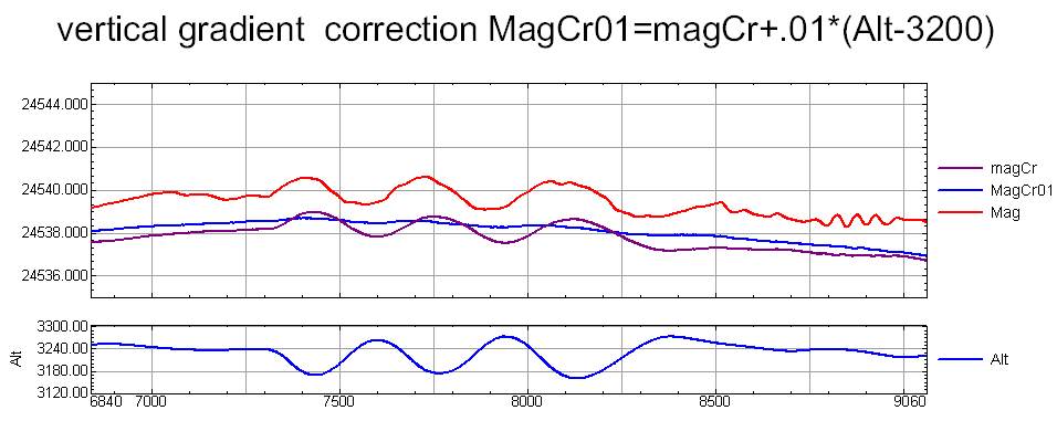
You have to understand that when making tuning changes the flight altitude and smooth curve appears only after adjusting the vertical gradient.
Here is the result of compensation from the sample.
Full-function trial version is
accessible with examples
You have to understand that when making tuning changes the flight altitude and smooth curve appears only after adjusting the vertical gradient.
Here is the result of compensation from the sample.
Two magnetic field sensors are installed on an aircraft. The quantum magnetometer measures the absolute value of the magnetic field with a high precision; the 3-axis flux gate magnetometer measures the magnetic field vector, but its precision is much lower. The quantum sensor can operate with a limited set of magnetic field directions only. There are three direction sets, where the quantum sensor fails to operate: his two poles and equator. When the aircraft flies above the Earth pole, the field direction is vertical, and its value is independent of the course (in the aircraft coordinates). Therefore, if the sensor is installed correctly, it will not leave the permissible orientation range, independently of the aircraft course. When the aircraft flies above the equator, only four orthogonal flight headings are permissible without changing the sensor orientation (along the tie-lines or along the traverse lines). The magnetometer axis shall be located at an angle of 45 degrees to the magnetic field direction. When setting the sensor orientation, the magnetic declination shall be taken into account, in addition to the route heading.
Hard Component
The aircraft causes magnetic field distortion of three types. The first distortion type (called a hard magnetic field component) is simply a constant additional vector component. The main vector may change its direction (in the aircraft coordinates); as the hard component is relatively low, the vector elongation is actually equal to the projection of the hard vector onto the main vector. If the reading of the vector magnetometer is normalized to unity, the considered correction is equal to the scalar product of the intrinsic magnetization vector by the normalized vector of the flux gate magnetometer.
Soft Component
The soft component results from the influence of the magnetic field on the aircraft parts, it depends on the direction of the external magnetic field. Additional magnetic field component appears in the point, where the quantum sensor is mounted; it is described by a 3´3 matrix. In order to determine its contribution to the resultant vector value, the projection of this component onto the main vector shall be found. As the result, a quadratic expression is obtained. Let us present this expression as a 3´3 matrix, whose above-diagonal elements are equal to zero. The elements X*Y and Y*X are equal to each other, they are determined together. As the result, 6 coefficients are obtained. It is again more convenient to use the normalized vector of the flux gate magnetometer; in this case, the correction will be proportional to the field, that is to the value measured by the quantum sensor. Thus, the coefficients obtain clearness and physical sense. When using the considered expression, it shall be multiplied by the field value in the given point and divided by the mean value at the moment of compensation (the difference between the real value and the measured value is neglected).
Let us assume, that the quantum sensor is enclosed into a uniform spherical shield, which reduces the magnetic field value equally in all directions. It is evident, that no experiments can help to determine the shielding factor. In other words, after including the compensation, the field values measured using different aircrafts are reducible to each other only to within a certain coefficient, close to 1. In addition, the aircrafts differ from each other, because the frequencies of their reference crystal oscillators used in the counters are different. Therefore, we must establish a certain additional condition. I assume, that the field directed along the axis X is true, so the corresponding correction is equal to zero. As the result, 5 coefficients remain.
Dynamic Component
The dynamic component accounts for the magnetic field induced by the currents, which arise, if the aircraft rotates in the terrestrial magnetic field (Foucault currents). This component is much lower, than those considered above. The dynamic component values are represented by a 3´3 matrix. The normalized flux gate magnetometer readings are used again; therefore, the obtained values shall be reduced to the actual magnetic field. The dimensionality (and the physical sense) of this matrix corresponds to the corrections, which arise, when the aircraft rotation speed is equal to one radian per a measurement cycle. It is supposed, that the magnetic field value varies rather slowly. We may assume, that the dynamic component arises, when a constant-length vector rotates in the aircraft coordinates (a normalized vector is used). Then the value X2+Y2+Z2 is constant, and ∂X*X+∂Y*Y+∂Z*Z=0. The diagonal matrix elements are interrelated through this expression; therefore, only two of them may be determined. The third coefficient may be accounted for, using the two elements found earlier. The upper left element is excluded from the calculation, it is assumed to be equal to zero. If another time step is used to calculate the difference in the flux gate magnetometer readings, the dynamic coefficients shall be corrected. The difference of the dynamic component from the other components is that its dimensionality is divided by radian per a measurement cycle. Fortunately, the aircraft does not rotate with such speed. So you shall not be confused, if the obtained values are of the order of tens or even hundreds. The dynamic component may be obtained through an individual channel; in this case, it will not be so high.
The measurement results are disturbed by the electrical noise onboard, thunderstorm, magnetic variation and instability of the reference crystal oscillator, used by the magnetometer counter. The influence of the rudders may be inspected on the ground; for one of aircrafts, the disturbance connected with the rudders corresponded to 0.4 nT. Before inserting the data into the program, the spike points (appearing mainly due to thunderstorm) shall be removed using standard Gesoft tools. The differential GPS system shall be used to obtain the coordinates.
Using the Program
The input text file has the Gesoft XYZ format. It contains the values obtained by means of the quantum sensor, three values obtained by means of the flux gate magnetometer, and three coordinates. The file may contain any number of lines. The line titles are read and sent to the output for the sake of statistics. Any row, which does not contain 7 numbers, is considered as the line break.
It is necessary to choose the number of used coordinates. A regime without coordinates is permissible, but the presence of numbers in 7 columns is necessary in any case. You may refuse to calculate the dynamic component, or to calculate both the dynamic, and the soft components.
The program operates with local data; it means, that displacing any line or shifting a level by a constant value does not influence the result. In this case, the length of 2 filters is specified. If there are no correlated disturbance factors for both sensors, the high-pass filter length may be set to zero. The low-pass filter separates the anomalous magnetic field from the influence of the evolutions.
At the output, we obtain the coefficients and some statistical data. The coefficients are given in the form of a table and in the form of a Gesoft expression (In geosoft script DIFF GX calculate differences between values in a channel and temporary variable is any name preceded by the '@' character.). The values obtained by the flux gate magnetometer (and normalized to unity), as well as their differences, are used in the expression. The script used for the calculations is given in the example (along with the templates for the input and output). A certain vertical gradient value is also sent to the output. This gradient value is used for the sake of control; the algorithm does not suppose a constant gradient.
Estimating the Results
The program has been used for 5 aircrafts during 2 years. The appended file is a typical file containing preliminary data without correction for the variation (the file is abbreviated for space saving). If the magnetic compensation is carried out in the considered example, the influence of the altitude on the magnetic field values is seen. The influence of the horizontal movement is not appreciable by eye, but it is also present. If the plots for the corrected and uncorrected values are compared, it seems, that the compensation has worked in some cases, but it has not worked in other cases. But if we use the correction command: +(Alt-3000)*0.011, we obtain another result, when it is impossible to detect the influence of the aircraft evolutions. As the program takes into account the evolutions in the space, the result shall reflect their influence (the evolutions include the aircraft movement upwards and downwards, as well as lateral displacement and velocity variation). The figure of merit (FOM) is not a reliable criterion for estimating the quality of the compensation. Another method for estimating its quality is based on flying through the same point with different headings. After the compensation is carried out, the variations are accounted for, and the correction for the altitude influence is made, the deviation of less than 1 nT is obtained. This value includes also various errors, in particular, the component, connected with remoteness of the base stations. It is impossible to estimate the actual error, but a numerical experiment may be easily carried out. Using the expression, given in the considered example, the distorted field is determined at first. We estimate the precision of the coefficients. If the compensation precision shall be estimated, the initial field shall be also used. But in the considered case it is not necessary, because we have set the coefficient values. The compensation result is given on the screenshot. We can see, that the calculated coefficients differ from the initial ones by 0.0001. The ratio of the initial hard vector to the residual vector equals to 100000. If the direction fluctuation is 0.1 radian, the fluctuation of the residual hard vector on the route is 0.00001. The ratio of the residual hard vector fluctuation on the route to the hard vector value is 1000000. The function given in the example is quite ordinary, its values and swing are similar to those of the actual magnetic field. Certainly, if a sinusoidal field distribution is given, whose period is close to the period of aircraft evolutions, the result will be much worse. There will be no background to filter the anomalous magnetic field.
The output data contain the parameter Gaus=0.1e-13; this parameter represents the solution conditionality. Its higher values correspond to more reliable solutions and lower disturbance influence. The solution based on field measurement using 4 headings is most reliable. Yet I can not recommend any particular Gaus value. This value may be enhanced by increasing the parameter of the low-pass filter. On the other hand, the influence of the surrounding field is increased in this case. I would recommend the filter length, which surpasses the evolution length by factor of 1.5 to 2. In the considered case, the filter length equal to 500 is more reliable, than 50. As a matter of fact, there is no basis for checking the accuracy of the compensation. The use of the FOM may indicate a low compensation quality in the worst case only. The geophysicist can estimate the final result only after plotting the maps. In opinion of the geophysicists, the obtained routes had initially insignificant deviation, and after a slight equalizing the result was excellent.